Postprocessings#

Postprocessings are metrics and tools that are available to analyze how your model is performing on your geometry.

Confidence Score#

The Confidence Score serves as an indicator of the AI model’s confidence in its predictions. This metric helps assess the reliability of predictions based on the underlying Gaussian Process (GP) uncertainty quantification. It is derived from the GP’s posterior variance at each mesh node.

What is a Confidence Score#

A 90% confidence score does not guarantee correctness but suggests the model has seen similar past patterns that led to this answer frequently.

A confidence score measures how certain the system is about its prediction, based on what it has learned from past data.

The score is calculated based on uncertainty scores for the output predicted by the model for this input. It is influenced by:

“Similarity/ Distance” to training examples in the input parameter space.
“Output variability”: even in regions with nearby training data, high variability can reduce confidence.

Legend:

The blue shapes represent the training data.
The red shape represents the prediction of interest.

This means that you might get low confidence even in the middle of well-predicted training points, if that region shows high output variability.

Conversely, high confidence can appear in distant regions if the model sees low variability and consistent behavior.

Being close to training data does not guarantee high confidence especially if that data had noisy outputs. The model can be uncertain in this region too.

What a Confidence Score is NOT#

A confidence score is not:

A prediction accuracy percentage.
A guarantee of simulation quality.
A statistical probability of correctness.
A direct measure of error magnitude

Interpreting Confidence Scores#

	High Confidence (example: 0.98)	Low Confidence (example: 0.40)
What it means	The model has seen very similar predictions during training.	This design is somewhat different from what the model was trained on.
What it does not mean	The model’s prediction is 98% accurate.	The prediction is 40% accurate and should be rejected.

Mean Normalized Width	Confidence Score	Interpretation
0.0	1.00	Perfect confidence - very tight intervals
0.1	~0.95	High confidence
0.5	~0.80	Good confidence
1.0	~0.67	Moderate confidence - intervals span prediction range
2.0	0.50	Low confidence - intervals are twice the prediction range

Best Practices#

Do	Do not
Use confidence scores to identify when predictions might involve extrapolation. View low confidence as a signal to add more training data in that region. Consider both confidence scores and prediction results together. Verify data quality when confidence patterns seem unexpected.	Assume high confidence guarantees accurate predictions. Always reject predictions solely based on low confidence (make further checks instead). Expect confidence to directly correlate with error magnitude. Use confidence score as the only validation metric.

How Confidence Scores Are Calculated#

The confidence score is a scalar value between 0 and 1 that aggregates nodewise uncertainty bounds into a single interpretable metric per geometry:

1.0 indicates highest confidence (minimal uncertainty).
0.0 indicates lowest confidence (maximum uncertainty).

2/3 (0.67) at the 95th percentile of the distribution. This means that 95% of training data have fewer uncertainty and will have a confidence score higher than 0.67 (and 5% lower than 0.67).
1 at the 5th percentile of the distribution. This means that 5% of training data have fewer uncertainty and will have a confidence score equal to 1 (and 95% lower than 1).

This calibration creates a meaningful scale:

Scores below 0.67 are labeled as “Low” confidence as it has a high uncertainty score compared to the scores of the training set.
Scores above 0.67 are labeled as “High” confidence as it falls within the range of the training set uncertainty scores.

Practical Application#

When developing models:

Start with an initial set of simulations.
Build a model and run predictions.
Identify areas with low confidence scores.
Add more training data in those specific regions if they are of interest to you.
Add more training data to the model to improve coverage and confidence and run the training again.
This iterative approach helps you efficiently develop robust models while minimizing the number of expensive simulations needed.

Global coefficients#

A Global coefficient is a numerical value that characterizes the overall behavior of an entire system. It helps understand how geometry behaves as a whole. These are scalar values that are automatically generated when the prediction is executed. The Global coefficients generated are calculated as defined during model configuration. They can be downloaded as JSON, CSV, and XLSX file formats. Example of Global coefficients: Drag, Lift.

Surface Postprocessing#

Some Surface postprocessing actions are available to you to either get a quick insight and indicators on the performance of your model or to download relevant outputs for further postprocessing outside of the Ansys SimAI Pro application.

With each prediction a new file is generated in the .vtp file format with the predicted field results selected as “Model Output” previously.

The data is either located at points or cells depending on which information was present in the training data set (in case of a mixed definition, the predominant occurrence is used). For each predicted field result the suffix “_pred” is appended to the name of the field.

For training on cell data, the prediction data are mapped onto the elements of the surface mesh. Hence, the coarseness of this mesh will affect the resolution of the exported prediction.

Table 1: Illustrations of the impact of the coarseness of the resolution of the exported prediction

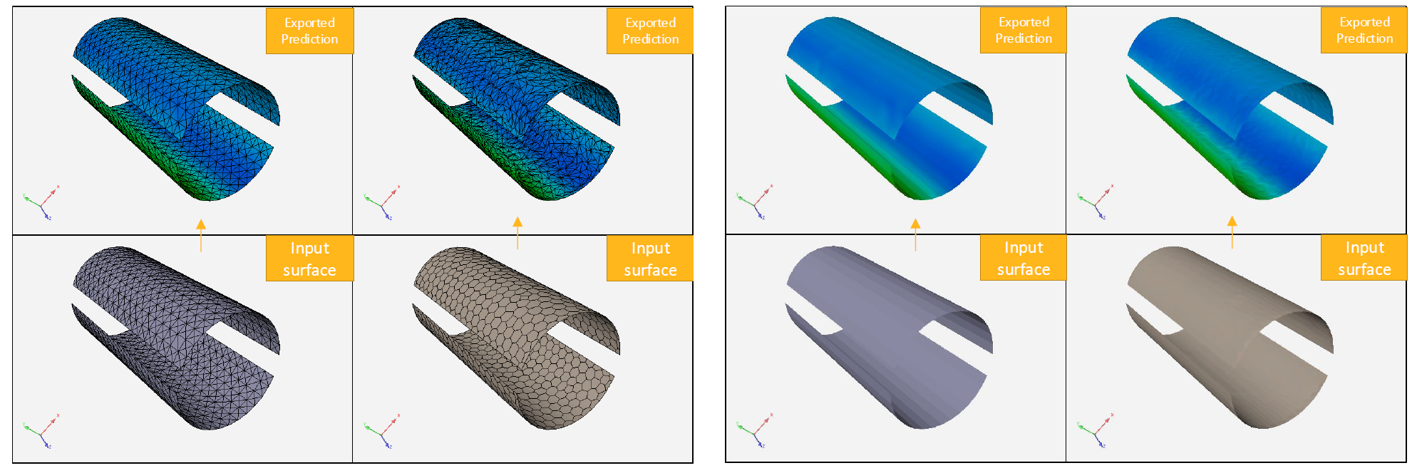
When all fields are generated at cells, they are mesh-agnostic in the sense that the field integral does not depend on mesh coarseness.

It is not the case when fields are predicted at points because the values depend entirely on the positions of the mesh nodes.

See Results#

The See results option allows you to start an interactive post-processor to visualize field results.

In case your data contains simulation results you can switch between the result and the prediction with suffix “_pred” to compare the prediction with simulation.

Download prediction#

With the Download prediction option you can save the .vtp file to your local file system to do further postprocessing outside the SimAI Pro application.

The exported .vtp file can be directly loaded in postprocessing tools such as the Ansys EnSight software to compare, script and treat the prediction like a regular simulation.